Table of Contents
This is the home page for Xanadu's quantum machine learning journal club. We will be working through an idiosyncratic syllabus on classical ML, in the hopes it will contribute to our expertise in QML, offer new insights or research approaches, and generally enhance our quality of life.
Here is the schedule (to be populated):
| Date | Material | Guide |
|---|---|---|
| Jan 9, 2024 | Admin | David Wakeham (DW) |
| Jan 23, 2024 | ESL: §2.1-2.4 | DW |
| (SVM: §1.1) | ||
| Feb 6, 2024 | ESL: §2.5-2.9 | Maria Schuld (MS) |
Notes on past meetings are in chronological order below.
1 Admin
Reading: None.
Based on popular accord, we'll be focusing on the classical statistical approach to ML embodied in Elements of Statistical Learning, and the effective field theory paradigm of The Principles of Deep Learning. These are like the out-of-field examiner and the scary departmental theorist at your viva. These foci will not stop us from being eclectic, and dipping into resources on Geometric Deep Learning, Support Vector Machines or Deep Learning proper, as time, interest, and chunking limits permit.
Each week we will have designated reading, optional readings (in
parentheses in the schedule), and a guide or guides who have agreed (or been
voluntold) to talk us through the readings. Notes will be uploaded here. For any
corrections, email <7@heptar.ch>.
2 Introduction
2.1 Statistical learning theory in brief
Reading: SVM: §1.1.
In statistical learning theory, our goal is to optimally approximate a function \(X \to Y\) using a training set of input-output samples, \[ \mathcal{D} = \{(x_{(1)}, y_{(1)}), \ldots, (x_{(n)}, y_{(n)})\}. \] A loss function is a map \(L: X \times Y \times Y \to [0, \infty)\) which measures how well \(f\) interpolates the data point \((x, y)\), with smaller values of \(L(x, y, f(x))\) as \(f(x)\) gets closer to \(y\). The expected loss or risk for a given \(f: X\to Y\), over the joint distribution \(P(x, y)\), is \[ \mathcal{R}(f) = \mathbb{E}[L(x, y, f(x))] = \int_{X\times Y} L(x, y, f(x))\, \mathrm{d}P(x, y). \tag{2.1} \label{risk} \] This is the average loss when we select an infinite number of pairs according to \(P(x, y)\). The empirical risk is the empirical approximation using our training pairs, \[ \mathcal{R}_{\mathcal{D}}(f) = \frac{1}{n}\sum_{i=1}^n L(x_{(i)}, y_{(i)}, f(x_{(i)})). \tag{2.2} \label{emp-risk} \] As \(n \to \infty\), the law of large numbers implies that \(\mathcal{R}_{\mathcal{D}} \to \mathcal{R}\), i.e. the empirical risk converges in probability to the risk. So for many data points, we can approximate this expected loss well. How do we learn the approximating function \(f\) based on these ideas? The minimal risk for a given loss function and distribution is \[ \mathcal{R}^* = \inf_{f: X \to Y} \mathcal{R}(f). \] Learning methods uniquely associate functions to training data, \(\mathcal{D} \mapsto f_{\mathcal{D}}\). The hope is that they approximate the minimal risk, \(\mathcal{R}(f_{\mathcal{D}}) \approx \mathcal{R}^*\), at least as our training set gets large. More formally, we say a learning method is universally consistent if \[ \lim_{n\to \infty} \mathcal{R}(f_{\mathcal{D}_n}) = \mathcal{R}^*, \] i.e. the function we learn minimizes risk.
In some ways, it's surprising such methods can exist for arbitrary distributions \(P\). In another way, it isn't, because we're only requiring asymptotic consistency, so we can gather enough data to map out \(P(x, y)\) to arbitrary accuracy. And indeed, the no free lunch (NFL) theorem states that, for any given speed of convergence (specified by a decreasing sequence), and any universally consistent learning method, there is some probability distribution which cannot be learned that quickly.
2.2 Linear and nonlinear regression
Reading: ESL: §2.3.
2.2.1 Linear regression
This is quite high concept, so let's dive into some specific methods for prediction, which also give us a sense of how statisticians think. One of the important tools in statistics is linear models aka linear regression. In the case our domain \(X = \mathbb{R}^p\), and \(Y = \mathbb{R}\), and we have reason to the inputs and outputs are linearly related, we can write \[ f(x) = \hat{\beta}_0 + \sum_{j=1}^p x_j\hat{\beta}_j = x^T \hat{\beta} \tag{2.3} \label{linmod} \] where \(x_j\) is the \(j\)-th component of the vector \(x\), and in the second equation, we have padded out \(x\) with a \(1\) in the zeroth component. The coefficients \(\hat{\beta}\) form a vector of \(p+1\) parameters (with the hat reminding us they are to be estimated from data), but we can extend this to a matrix for \(Y = \mathbb{R}^k\). For the moment, let's keep \(k=1\), and absorb the padding into \(p\).
As before, we would like to pick the best \(\beta\) for our data using a loss function. A natural and in some sense optimal choice for linear models is called the residual sum of squares, where the loss function is just squared distance: \[ L(x, y, f(x)) = |y - f(x)|^2 = |y - x^T \beta|^2. \] Let \(\mathbf{y} = (y_{(i)})^T\) be a column vector of \(n\) training outputs, and \(\mathbf{X} = (x_{(i)}^T)\) an \(n\times p\) matrix of training inputs. The empirical risk \((\ref{emp-risk})\) can then be written \[ \mathcal{R}_{\mathcal{D}}(\beta) = \frac{1}{n}\sum_{i=1}|y_{(i)} - x_{(i)}^T\beta|^2 = \frac{1}{n}(\mathbf{y} - \mathbf{X}\beta)^T (\mathbf{y} - \mathbf{X}\beta). \tag{2.4} \label{RSS} \] We can solve this for the optimal \(\beta\), simply by differentiating with respect to \(\beta\): \[ \partial_\beta \mathcal{\mathcal{R}_{\mathcal{D}}(\beta)} = \frac{1}{n}\left[\mathbf{X}^T\left(\mathbf{X}\beta -\mathbf{y} \right) + \left(\mathbf{X}\beta -\mathbf{y} \right)^T \mathbf{X}\right] = \frac{2}{n}\mathbf{X}^T\left(\mathbf{X}\beta -\mathbf{y}\right), \] where the last equality follows from the fact that a scalar is its own transpose. More carefully, we can differentate either component-wise, or with respect to both \(\beta\) and \(\beta^T\) as formal variables. Assuming \(\mathbf{X}^T\mathbf{X}\) has an inverse, we can set this to zero and solve for \(\beta\): \[ \mathbf{X}^T\left(\mathbf{X}\beta -\mathbf{y}\right) = \mathbf{X}^T\mathbf{X}\beta -\mathbf{X}^T\mathbf{y} = 0 \quad \Longrightarrow \quad \hat{\beta} = (\mathbf{X}^T\mathbf{X})^{-1}\mathbf{X}^T\mathbf{y}. \tag{2.5} \label{beta-hat} \] Again, the hat tells us that we estimate this from data.
Let's look at an example. Below, we have a scatterplot of \(100\) simulated data points on a pair of inputs, \(x = (x_1, x_2)\). The output is a categorical binary variable, i.e. \(0\) and \(1\), indicated by \(\textcolor{blue}{\texttt{o}}\) and \(\textcolor{orange}{\texttt{o}}\) in the scatterplot. We can fit a linear regression model to the data, with a real variable \(y\) which gets coded as \(0\) when \(y \leq 0.5\) and \(1\) otherwise. In other words, we have a linear decision boundary at \(y = x^T\hat{\beta} = 0.5\), where \(\hat{\beta}\) is given by \((\ref{beta-hat})\).
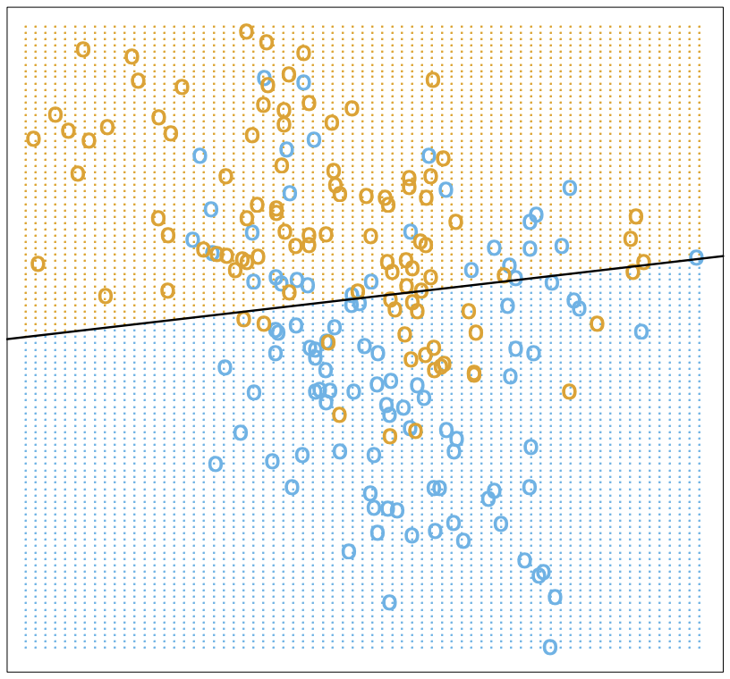
There are misclassifications, but whether our model is good or bad depends strongly on our assumptions about the data. Consider two possibilities:
- The data comes from two independent bivariate Gaussian and different means.
- The data comes from a mixture of \(10\) low-variance Gaussians, with means distributed in a Gaussian fashion.
In the first case, the data is, in fact, optimally described by a linear decision boundary (bisecting the means of the component Gaussians) but inevitably noisy. In the second case, we have clusters, so a linear decision boundary will do poorly on future data. Let's turn to a nonlinear method that does better in this second scenario.
2.2.2 Nearest neighbours
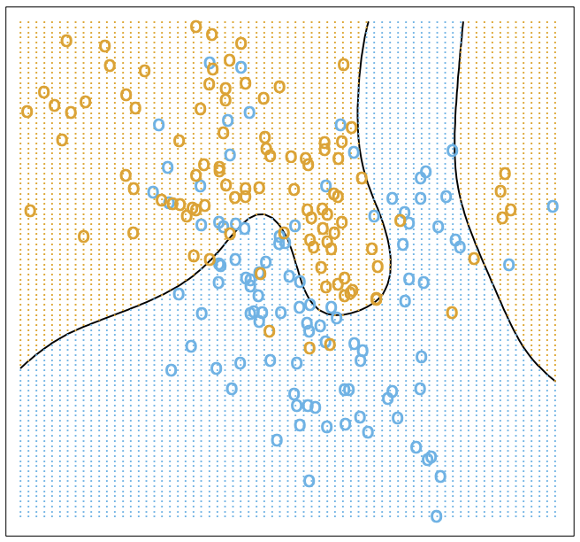
Nearest neighbours is a very different approach. The idea is that is simply to approximate the value of response variables for a new data point by averaging the values of its nearest neighbours in the training data \(\mathcal{D}\). Let \(N_k(x)\) denote the \(k\) nearest neighbours of \(x\). Then our \(k\)-nearest-neighbour regressor is \[ f(x) = \frac{1}{k}\sum_{x_{(i)} \in N_k(x)} y_{(i)}. \] Closeness will mean in Euclidean distance, but could of course be generalized to an arbitrary metric space. In our binary case, this boils down to a majority vote. This is a much less rigid method than linear regression, so when we fit our binary-coded data, we get a much wobblier decision boundary \(f(x) = 0.5\). Below, we show \(k = 15\):
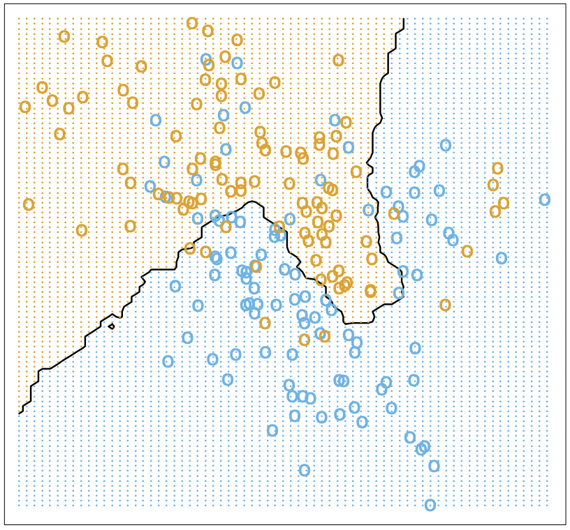
We have fewer misclassifications, but of course, we can easily overfit with nearest neighbours. For instance, with \(k=1\) there are no misclassifications, by definition! So to determine the appropriate choice of \(k\), we need a test set and a method besides minimizing empirical risk. Note that to count parameters, we should use \(n/k\) (where \(n = |\mathcal{D}|\)) rather than \(k\), since this is the number of clusters it gloms our data into.
To get test data, we need to open up the data-generating black box. The data is generated hierarchically as follows: we have two Gaussian distributions of Gaussians, with ten means drawn from one distribution (centred at \((1, 0)^T\)) and ten from another (centred at \((0, 1)^T\)), forming our two different classes (\(\textcolor{blue}{\texttt{o}}\) and \(\textcolor{orange}{\texttt{o}}\)). Each mean had a small Gaussian centered on it, and from the two classes, Gaussians were chosen at random to draw observations from. We can see how methods perform on a test set:
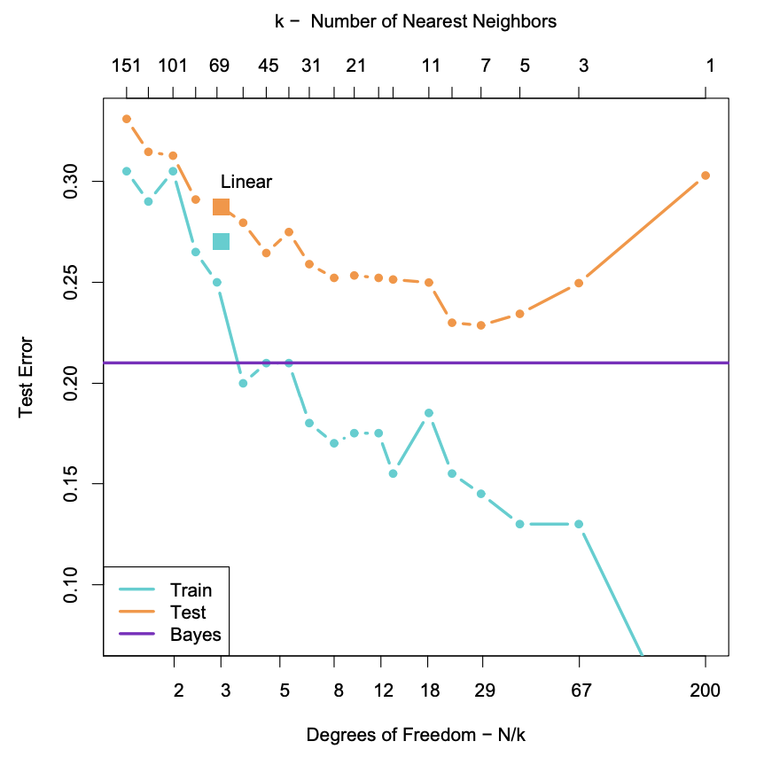
The purple line is the optimal Bayes error (to be discussed below). The two large squares are the results of linear regression, which has three degrees of freedom. The curves are results for nearest neighbours, with \(n/k\) increasing to the right. Interestingly, it performs as well as linear regression for the same number of parameters, with lower training error. How can we get a handle on these two methods?
2.3 Regression and statistical learning
Reading: ESL: §2.4.
2.3.1 Conditional mean
Let's return to the statistical learning theory we began to explore above, but with our two examples in mind. We will focus on squared error loss in the risk \((\ref{risk})\). If we condition on \(x\), using the definition of conditional probability \(P(x, y) = P(y|x)P(x)\), then \[ \mathcal{R}(f) = \mathbb{E}[L_2(x, y, f(x))] = \mathbb{E}[(x - f(y))^2] = \mathbb{E}_x\big[ \mathbb{E}_{y|x} [(y - f(x))^2 | x]\big]. \] To minimize the expectation of a function over \(x\), it suffices to minimize it pointwise, i.e. for each \(x\), we want to choose \[ f(x) = \mbox{argmin}_c \mathbb{E}_{y|x} [(y - c)^2 | x]. \] To minimize this, note that \[ \partial_c\mathbb{E}_{y|x} [(y - c)^2 | x] = \partial_c\int_{y\in Y} (y-c)^2 \,\mathrm{d}P(y|x) = 2\int_{y\in Y}(c-y) \,\mathrm{d}P(y|x) = 2c - 2\mathbb{E}_y[y|x]. \] Setting this to zero, we should take \[ f(x) = \mathbb{E}_y[y|x]. \tag{2.6} \label{regress-f} \] This is called the regression function, and it tells us that to minimize expected squared loss, we should choose the conditional mean. Of course, we could use a different loss function, say absolute value \[ L_1(x, y, f(y)) = |y - f(x)| \] instead, and the same argument would give the conditional median \[ f(x) = \mbox{argmin}_c \mathbb{E}_{y|x}[|y - c|\, | x]. \] However, we'll continue focusing on squared loss.
2.3.2 Revisiting methods
Nearest neighbours approximates the conditional mean directly. First, it uses empirical probabilities rather than the underlying distribution, since it only has access to the latter, which we can write as \[ \mathbb{E}_y[y|x] \approx \mbox{Ave}\{y | (x, y) \in \mathcal{D}\}, \] where \(\text{Ave}\) is a sum divided by the number of summands. Second, since data is usually sparse, we replace conditioning on \(x\) for conditioning on a neighbourhood \(N(x)\) of \(x\): \[ \mbox{Ave}\{y | (x, y) \in \mathcal{D}\} \approx \mbox{Ave}\{y|(x', y) \in \mathcal{D}, x' \in N(x)\} = \hat{f}(x), \] where the last expression is the nearest neighbours regressor. Provided the distribution is approximately locally constant, as \(n/k \to \infty\) these approximations are good, and \[ \lim_{n/k \to \infty} \hat{f}(x) = \mathbb{E}_y[y|x]. \] So we have a universal approximator! The problem is, as we might expect from the NFL theorem, the method can be unstable, inapplicable because \(n\) is too small, or extremely slow for e.g. dimensional reasons, as we'll discuss soon.
Linear regression is a more explicit model-based approach, where we assume our data is approximately linear: \[ f(x) \approx x^T\beta. \] If we plug this into our risk function, and differentiate with respect to \(\beta\), we find \[ \partial_\beta\mathcal{R}(\beta) = \partial_\beta\mathbb{E}[(y - x^T\beta)^2] = 2 \mathbb{E}[x(y - x^T\beta)]. \] Hence, we get \[ \beta = \mathbb{E}[xx^T]^{-1}\mathbb{E}[xy], \] which we approximated earlier using training data in \((\ref{beta-hat})\). So, in contrast to nearest neighbours which works on locally constant functions, linear regression works on globally linear functions. Both approximate the conditional mean, but in different ways.
2.3.3 Bayes classifier
We have coding categorical variables using a regressor, but we can introduce a risk function explicitly adapted for classification. If our categorical variables take values in some set \(c_i \in C\), we can store the penalties for classifying an observation in class \(c_i\) as \(c_j\) in a matrix \(L(c_i, c_j)\). An example is the \(0\)-\(1\) loss \(L(c_i, c_j) = 1 -\delta_{ij}\), where misclassifications cost one unit of loss. The risk is \[ \mathcal{R}(f) = \mathbb{E}[L(c, f(x))], \] where expectation is with respect to \(P(c, x)\). Again, by conditioning on \(x\), minimizing risk becomes pointwise minimization: \[ \hat{c}(x) = \mbox{argmin}_{c \in C} \sum_{k=1}^{|C|} L(c_k, c) P(c_k | x). \] With the \(0\)-\(1\) loss, this becomes \[ \hat{c}(x) = \mbox{argmin}_{c \in C} \left[1 - P(c |x)\right] = \mbox{argmax}_{c \in C} P(c |x). \tag{2.7}\label{bayes-class} \] This is called the Bayes classifier, and it instructs us to classify to the most probable class given the conditional distribution over \(x\).
Above, we show the Bayes optimal decision boundary, i.e. the crossover point \[ \{x : P(\textcolor{blue}{\texttt{o}}|x) = P(\textcolor{orange}{\texttt{o}}|x)\} = 0.5 \] in the conditional distribution. Nearest neighbours gives a local estimate of this conditional distribution from the neighbourhood majority vote, so we have yet another way to think about what nearest neighbours does.
3 References
- Elements of Statistical Learning (2008), Hastie, Tibshirani and Friedman. [ESL]
- The Principles of Deep Learning (2021), Roberts and Yaida. [PDL]
- Geometric Deep Learning (2021), Bronstein, Bruna, Cohen, and Veličković. [GDL]
- Support Vector Machines (2008), Steinwart and Christmann. [SVM]
- Deep Learning (2015), Aaron Courville, Ian Goodfellow, and Yoshua Bengio. [DLB]