March 8, 2026. Sparse autoencoders (SAEs) are a crucial mechanism for extracting interpretable information from a neural network. In this post, we explore the decay of recoverability with the size of the SAE, guided by work from compressed sensing.

Inspired by the research from Anthropic’s mechanistic interpretability group, I decided to explore the statistical physics of sparse recovery in neural networks. Following the experimental trail and theoretical cues from Donoho and Tanner, we will identify what looks like universality in the behaviour of recoverability and suggest guidelines for SAEs in practice.

Contents

1. When Bigger is not Better
2. Setting it Up
3. Hunting the Crossing
4. Thoughts and Open Questions

---

1. When Bigger is not Better

Machine learning models play an increasingly important role in our lives, but are notoriously opaque. An archetypal example is neural networks, which can be hard to interpret since neurons often fire for unrelated reasons; a single neuron might respond to fragments of Korean, HTML, and references to Teenage Mutant Ninja Turtles. This baffling behaviour is called polysemanticity (“many meanings”) and occurs when feature activation patterns are sufficiently sparse; in this case, it makes sense to use the same neuron for different purposes, since those purposes (approximately) don’t interfere with each other. To learn features in an interpretable way, we can train sparse autoencoders (SAEs) on those networks. I’ll explain how that’s performed technically in the next section, but loosely speaking, we encourage the SAE to learn one feature per (SAE) neuron. Thus, the SAE acts like a semantically “unfolded” version of the original neural network.

But how do we know we’ve captured the meaning of the original network, $\mathcal{N}$? Suppose we have $N$ neurons in $\mathcal{N}$ and $F$ neurons in the SAE $\mathcal{F}$ we are training. We naturally want $F > N$, in order to disentangle the different features the neurons in $\mathcal{N}$ are activated by. But how much bigger is ideal? It turns out there is a tradeoff between our ability to disentangle activations, which pushes us in the direction of bigger $\mathcal{F}$, and the information we can extract from $\mathcal{N}$, which pushes towards smaller.

The latter point is a little counterintuitive. Basically, the larger $\mathcal{F}$ is, the more ways it provides to explain a given activation pattern; to select a unique explanation, we use sparsity as a tie-breaker. After a point, though, there are too many sparse vectors consistent with the observed pattern of activity that information about $\mathcal{N}$ gets lost, like a needle in a haystack. This raises a concrete architectural question: how big should our SAE be? We’ll experiment with a synthetic toy model where we can track how recoverability behaves.

2. Setting it Up

Our “trained” neural network $\mathcal{N} = \mathbb{R}^N$ consists of $N$ neurons, while the SAE $\mathcal{F} = \mathbb{R}^F$ will have $F > N$ feature neurons. We let $\alpha = F/N$ denote the ratio of dimensions, and assume $k$-sparsity, with $k = \rho F$ features activated at a time for a ratio $\rho = k/F \in [0, 1]$ that we will vary. The weights of the trained network are represented by a ground truth encoding $W: \mathcal{F} \to \mathcal{N}$; this is automatically polysemantic, since it crams a large feature space into a physically smaller set of neurons. Given a feature vector $f \in \mathcal{F}$, the neuron activations are simply

\[n = Wf \in \mathcal{N}.\]

The SAE’s job is to invert this, and recover a guess $\hat{f}$ from $n$. Since $F > N$, the map $W$ is not injective, so many feature vectors produce the same activation pattern and naive inversion is hopeless. Sparsity is the tie-breaker. If we know $f$ has at most $k$ nonzero entries, the problem becomes well-posed, at least in principle. Technically the number of nonzero entries is counted by the $\Vert\cdot\Vert_0$ norm, but because this behaves discontinuously, we enforce sparsity with the next best thing, the $\Vert \cdot\Vert_1$ norm which counts the sum of sizes of entries:

\[\ell(n, \hat{f}) = \Vert n - W\hat{f}\Vert_2^2 + \lambda \Vert \hat{f}\Vert_1, \tag{1}\label{lasso}\]

where $\hat{f} = \hat{V}n$ for a learned mapping $\hat{V}:\mathcal{N}\to \mathcal{F}$ called the SAE decoder.

With this setup in hand, we can ask when recovery is possible. There is a natural threshold at $\alpha = 1$. Below this point, $W$ is generically injective, since there are more neurons in $\mathcal{N}$ than features in $\mathcal{F}$. Thus, a linear decoder (technically speaking, the pseudoinverse $W^+$) suffices. Above $\alpha = 1$ however, the nullspace of $W$ becomes nontrivial; inevitably, some nonzero vectors are annihilated, corresponding to feature directions which are invisible in $\mathcal{N}$. No linear decoder can recover. This is where polysemanticity starts, and our sparsity tie-breaker comes into play in order to select $\hat{V}$. The question is whether there is structure beyond the simple $\alpha = 1$ threshold.

3. Hunting the Crossing

Onto the experiments. In our synthetic setup, features and encodings are described as follows:

• $W$ is a Gaussian random matrix with normalized columns;
• features $f$ are drawn from a Bernoulli-Gaussian distribution, where an entry is nonzero with probability $\rho = k/F$ and then distributed as $\mathcal{N}(0, 1)$.

This is simple enough to model easily (and even reason about analytically), but complex enough to give rise to polysemantic behaviour. We compare two different decoders:

• the linear decoder or pseudoinverse $W^+$, which obeys $WW^+ = I$;
• the linear map trained with loss (\ref{lasso}), a procedure called the LASSO, with $\lambda$ calibrated to target the sparsity $k$ at a given $(\alpha, \rho)$.

The first is a naive but useful baseline, while the second is the target we train in practice. Finally, we measure two complementary accuracy metrics:

• the support recovery accuracy (SRA), the fraction of true nonzero entries of $f$ that appear in $\hat{f}$;
• the normalized mean-squared error (MSE), the expected value of $\Vert f - \hat{f}\Vert_2^2/\Vert f\Vert_2^2$ over $f$.

SRA is something like a $\Vert \cdot\Vert_0$ measure of accuracy while the MSE corresponds to $\Vert \cdot\Vert_2$. Our first experiment explores how these metrics change with $\alpha = F/N$, sweeping $\alpha$ from $0.4$ to $6.5$, holding $N=200$ and varying $\rho\in \lbrace 0.05,0.10,0.20\rbrace$. Here are the plots:

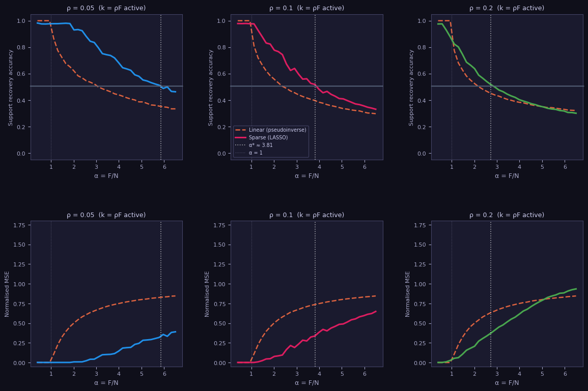
As we expect, the linear decoder quickly degrades beyond $\alpha = 1$, while the sparse LASSO decoders also decay more quickly as $\rho$ increases, or put differently, sparsity decreases. This makes sense too; the denser features are, the harder to disentangle! But there is a mysterious consistency lurking in these plots. Although the LASSO curves behave differently, they also cross $\text{SRA} = 0.5$ (indicated by a solid line) for a special function of $\rho$ (thicker dotted line):

\[\alpha^\ast(\rho) = \frac{1}{C\rho \log(1/\rho)}, \quad C \approx 1.14. \tag{2} \label{DT}\]

This sensibly diverges as $\rho \to 0$; we expect this, since any number of neurons should be able to recover features that never co-occur. The existence of this “transition” suggests universality underlying the behaviour of the sparse decoder, parametrized by $\rho$. (The universality for the MSE is still present but weaker, so we focus on the SRA.)

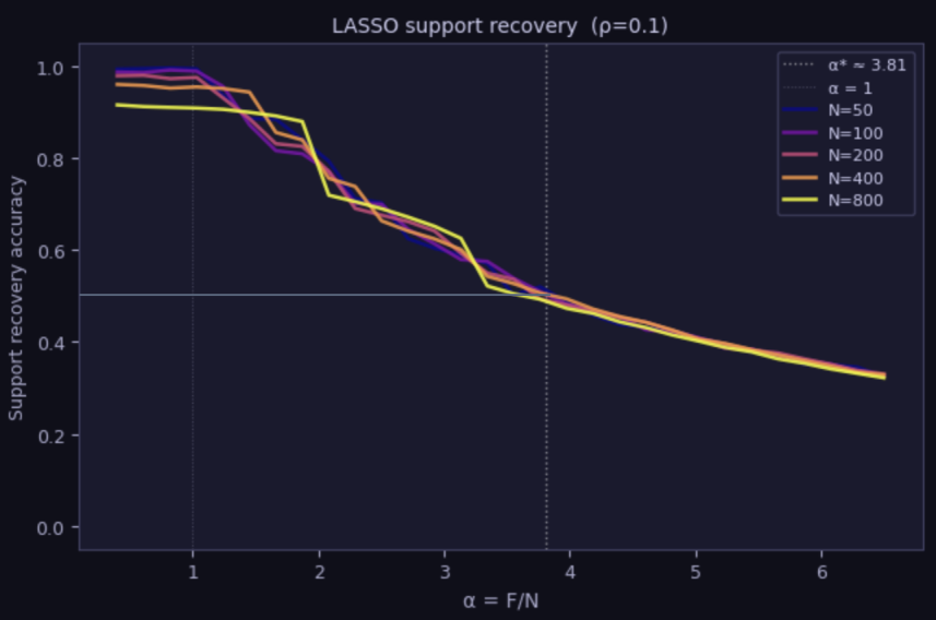
Another probe of universality is to vary $N$ and see how the curves fluctuate; if the behaviour is universal, we would expect to see crossing at the same value. Here, we plot the LASSO SRA for $\rho = 0.1$ and various values of $N$. The results initially fluctuate due to finite-size effects, but settle into a universal crossing right around the $\text{SRA} = 0.5, \alpha^\ast \approx 3.81$ mark:

Solving a sparse recovery problem puts us in the setting of compressed sensing, where foundational results in the literature tell us the LASSO is not optimal (though it is performant). Instead, near-optimality is guaranteed for a method called basis pursuit. We defer the details to the next section, but here, simply compare a basis pursuit algorithm called FISTA to LASSO:

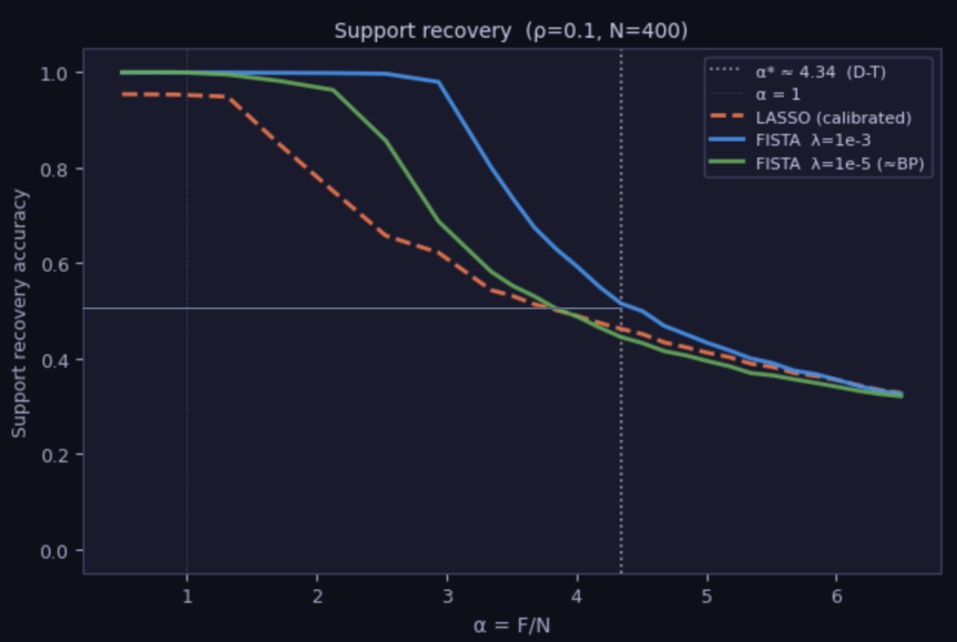
The punchline is that by tuning the regularization constant $\lambda$ in FISTA, we can outperform LASSO decoding and hit $\text{SRA} = 0.5$ at a higher $\alpha$ corresponding to $C = 1$ in (\ref{DT}). We conjecture this is optimal.

4. Thoughts and Open Questions

Why does the crossing occur at $\alpha^\ast(\rho)$? The answer comes from compressed sensing, which studies the problem of sparse recovery $n = Wf$. The basic idea is that, when there are $k$ nonzero entries for a vector in $\mathcal{F}$, there are $\binom{F}{k}$ ways to choose the “active” dimensions, and hence the active subspace $f$ (or rather, our reconstructed $\hat{f} = \hat{V}n$) lives in. If we knew which subspace $W$ lived in, we could easily invert by restricting to those $k$ columns. The problem is that we don’t know the subspace, and to determine it takes roughly

\[N^* \approx \log \binom{F}{k} \approx k \log (F/k)\]

measurements, using Stirling’s approximation, where we treat each neuron activation $n_i = w_i \cdot f$ as a single linear measurement of the feature vector. This leads to

\[\alpha^* = \frac{F}{N^*} = \frac{1}{k \log (F/k)} = \frac{1}{\rho \log(1/\rho)}\]

as claimed. This is closely related to the combinatorial phase transition observed by Donoho and Tanner (2009). See their paper for a more precise geometric argument.

What does this mean for SAE design? We focused on the Gaussian random situation after Donoho and Tanner. We don’t know if our recoverability results apply to real neural networks, but assuming they do, it suggests that we may want to train with something other than the LASSO, with a tuning problem to solve for the theoretically optimal basis pursuit method. We did a $\lambda$ sweep for different values of $\alpha$, and found the optimal value varies over orders of magnitude:

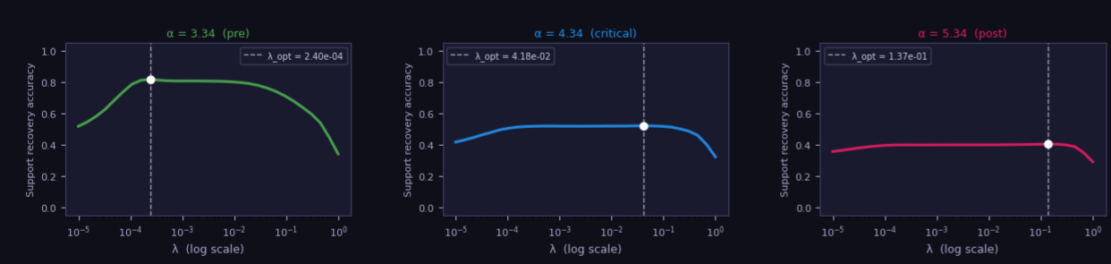
That seems like bad news for the regularization schedule. Luckily, the curves are forgiving, with a broad near-optimal plateau in the middle that falls off either side. If we stick to that plateau, we should be good. If $C=1$ is optimal and universal, it tells us there are hard limits to recoverability. Although expanding the SAE can initially yield finer-grained feature sets, at some point, we will start to lose information from the original network as it gets diluted irrecoverably into the many subspaces. Our findings suggest that, as a design principle, we should consider the tradeoff between feature grain and information loss carefully.

What is basis pursuit? The LASSO decoder minimises $\ell(n,\hat{f})$ from equation (\ref{lasso}) with a finite $\lambda$, which introduces a bias, since it shrinks all coefficients toward zero, not just the inactive ones. The theoretically optimal sparse decoder is basis pursuit, which takes $\lambda \to 0$ while enforcing the constraint $W\hat{f} = n$ exactly:

\[\min_{\hat{f}} \Vert\hat{f}\Vert_1 \quad \text{subject to} \quad W\hat{f} = n.\]

This looks harder, since it’s a constrained optimization rather than a penalized one, but the remarkable fact, proved by Candès, Romberg and Tao (2006) and Donoho (2006), is that this convex program recovers the true sparse $f$ exactly whenever $N \gtrsim k\log(F/k)$. No bias, no shrinkage, no tuning of $\lambda$. In practice, basis pursuit is solved iteratively and approximately using FISTA (Fast Iterative Shrinkage-Thresholding Algorithm), which still has a sparsity term regularized by $\lambda$, and approaches basis pursuit exactly as $\lambda \to 0$. As discussed in the previous point, for reasons that are not entirely clear, the optimal $\lambda$ is somewhat finely tuned, and neither pure basis pursuit nor LASSO saturate $C = 1$.

Black holes? The secret underlying this post is that everything here was inspired by thinking about neural networks as black holes. I’ll expand on this more in a future post, but the basic observation is that black holes scramble and leak information into auxiliary systems surrounding the black hole, much as $\mathcal{N}$ scrambles and leaks information into $\mathcal{F}$. There are constraints on how and when we can access information called the Page curve; I simply wanted to find the Page curve of training an SAE.

Code

See GitHub for the code that generated the plots.

Acknowledgements

This post was developed in collaboration with Claude (Sonnet 4.6), which contributed to experimental design, numerical implementation, and theoretical content.